Newsroom
Booting Fast and Slow
At H Company, our agents are served by a fleet of vLLM replicas running on GPU nodes in Kubernetes.
July 8, 2026 · 19 min readBy Emrick Sinitambirivoutin, Victor Goubet, Avshalom Manevich
At H Company, our agents are served by a fleet of vLLM replicas running on GPU nodes in Kubernetes. Agentic workloads are bursty, so being able to dynamically adjust our number of replicas is key, and that adjustment is only as fast as the time it takes a new replica to become ready.
For our largest models, this process previously took up to 27 minutes. Every minute spent waiting translates directly to increased latency for our users or forces us to keep GPUs active "just in case" to avoid the wait. Boot time also taxes everything else we do: deployment rollouts, RL training jobs that spin up inference servers, and research iteration speed all sit behind the same cold-start wall.
To enable effective autoscaling, we distinguish between two startup scenarios:
- Cold start: Occurs when we deploy a model configuration for the first time.
- Warm start: Occurs when we scale up an existing deployment or during the consecutive phases of a rolling update.
This post details our efforts to optimize every layer of the stack, achieving up to 3x speedup in the cold start and 12x end-to-end speedup in the warm start scenario for a Qwen3.5 397B-A17B FP8 model.
 (opens full size in a new tab)
We will cover the following areas of improvement that we worked on:
- Implementing end-to-end deployment traces by contributing OpenTelemetry (OTEL) startup tracing to vLLM.
- Eliminating Docker pulls from the critical path using a DaemonSet-based image cache.
- Leveraging NVIDIA ModelExpress model streamer to have a 3x speedup in weight pulling from S3.
- Transitioning to GPU-to-GPU RDMA transfers at 341 Gbps via AWS EFA and ModelExpress, including an upstreamed fix for silent TCP fallbacks and the addition of OTEL tracing support.
- Achieving a 4x to 5x warmup speedup by sharing FP8 compilation caches across replicas.
In summary, these enhancements enable us to improve cold boot speeds by 3x and achieve up to a 12x acceleration for warm boots.
The problem
While the engine itself is critical, a vLLM replica spends a significant portion of its lifecycle in the orchestration layers before initialization even begins. To capture this, we augmented our vLLM main image metrics with deployment-level tracing in Datadog. By monitoring pod scheduling, Docker image pulls, and the execution of both init and main containers, we gain a comprehensive end-to-end perspective, from the moment a "Pod is created" until it is "Ready to serve."
The startup process for a vLLM replica is essentially a four-stage sequence:
- Docker Image Pull: Retrieving the heavy vLLM image from ECR.
- Weight Acquisition: Staging the necessary model weights from S3 onto the local node.
- Engine Initialization: Executing Python imports and moving weights into GPU memory.
- CUDA Warmup: Performing CUDA graph capture and JIT kernel compilation, specifically for DeepGEMM in FP8.
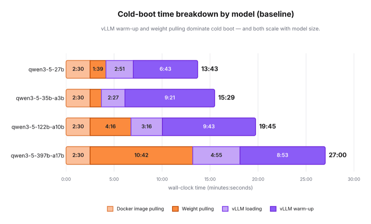
Here is what the baseline looks like on the Qwen3.5-VL family with vLLM 0.19.1:
 (opens full size in a new tab)
Cold-boot time breakdown by model at baseline.
This performance baseline highlights three primary areas for improvement:
- Image pull fixed tax: Cold pulls for new tags add a flat 2 minutes 30 seconds to the process. While this is under 10% of the boot time for the 397B model, it hits the smaller 27B instance with an 18% delay.
- Linear weight scaling: Staging time climbs alongside model size. Downloading the weights takes 1 minute for the 27B variant but stretches to nearly 11 minutes for the 397B FP8 model.
- The warmup penalty: DeepGEMM JIT compilation adds severe overhead to FP8 warmup. It is the worst bottleneck for smaller models, taking up to 58% of the boot timeline for the 35B version.
Our Multi-Layered Approach for Fast(er) Horizontal Scaling
Layer 0: Observability
Initially, our observability was limited. We operate by the principle that we can only improve what we can measure, but our previous setup relying on brittle log scraping left critical phases obscured.
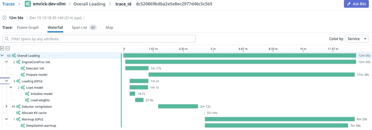
To address this, we integrated OpenTelemetry startup tracing into the vLLM upstream. This contribution introduces spans for engine initialization, weight staging, GPU warmup, CUDA graph capture, and compilation, ensuring trace context is maintained across worker processes.
 (opens full size in a new tab)
Figure 1: Trace visualization of the vLLM loading phase.
However, since a replica's lifecycle begins well before the engine starts, we expanded this with deployment-level tracing via Datadog.
This broader view captures pod scheduling, container execution, and image pulling. The result is a comprehensive end-to-end trace for every deployment, tracking progress from "Pod created" to "Ready to serve", which provides the data foundation for the benchmarks presented in this post.
Layer 1: Taking image pulls off the critical path
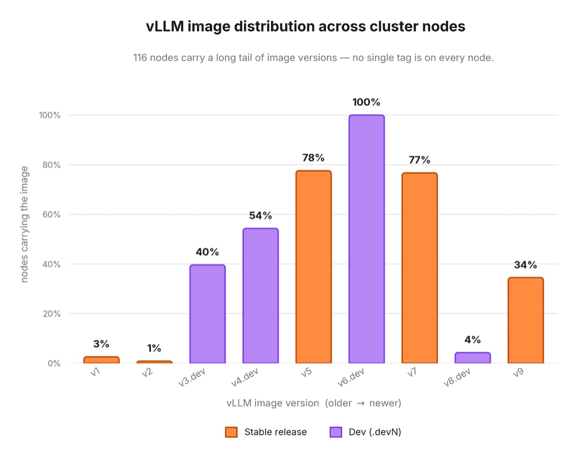
Each deployment references a versioned vLLM image. kubelet pulls images reactively: a tag only lands on a node when a Pod referencing it is scheduled there. Across a large cluster with a handful of concurrently active vLLM versions, this produces a sparse, asymmetric distribution. Each node accumulates only the versions that happened to land on it, and any deployment scheduled onto a node missing the tag pays a multi-GB cold pull before vLLM can even start.
 (opens full size in a new tab)
Figure 2: vLLM image distribution across cluster nodes.
In figure 2, we can see one of the newest images (v8.dev) is present on only 4% of nodes, so a fresh deployment almost certainly paid the pull.
The fix uses a DaemonSet to pre-pull images directly onto the inference nodes. It requires no third-party tools and works without modifying your existing deployment definitions.
- Node targeting: The configuration applies to inference nodes by matching node selectors for the GPU type and affinity rules for the workload pool, along with the required tolerations.
- Image pulling and retention: The spec configures 1 init container for every target image to handle the download to the node. Once those exit, a main container running a pause image keeps the pod alive while drawing a negligible resource floor of 10m CPU and 32Mi memory.
The caching relies on standard kubelet scheduling. The node has to pull the image before it can run the container, which leaves the layers in local storage once the init container exits.
Adding a new image version takes a single-line change in the DaemonSet config. From there, deployments on that node skip the ECR pull completely, cutting around 2 minutes 25 seconds off the average cold start.
Layer 2: Optimizing weight pulling from S3
Weight staging is the primary bottleneck in our deployment pipeline for large models. The baseline configuration takes nearly 11 minutes just to stage the weights for a 397B FP8 model.
 (opens full size in a new tab)
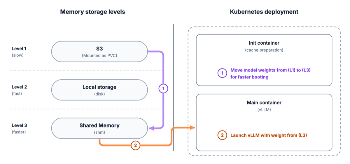
Figure 3: Baseline deployment implementation.
Our baseline flow described in Figure 3 is:
- An init container copies weights from an S3 File System in UserSpace (FUSE) mount into a tmpfs volume in
/dev/shm. - The main vLLM container starts. The vLLM loader reads from tmpfs into pinned host buffers and runs a
cudaMemcpyto the GPUs.
This setup suffers from two structural flaws and one embarrassing execution detail. First, every replica re-downloads from S3 because there is no peer sharing mechanism. Second, the weights occupy a full extra copy in host RAM. Finally, the execution uses a plain cp command, which results in a single threaded read through FUSE.
Before optimizing, we calculated our theoretical bandwidth limits. A p5.48xlarge instance has 3,200 Gbps of aggregate network capacity. However, IP traffic is capped at 800 Gbps, and single IP traffic drops to a usable 100 Gbps. This leaves a realistic ceiling of about 12.5 GB/s for a single node S3 download.
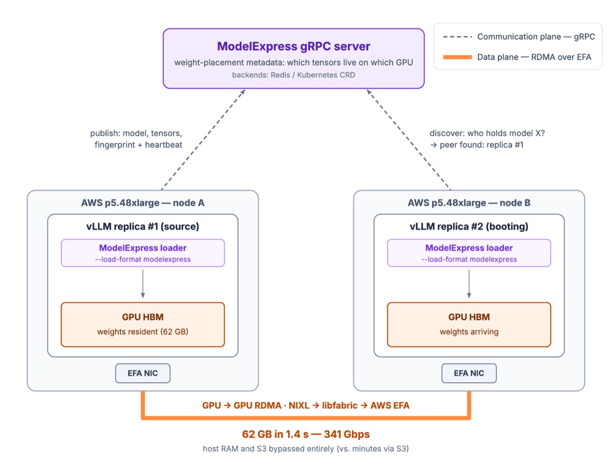
To hit this ceiling, we removed the init container and shifted weight loading to ModelExpress, an open source (Apache 2.0) project from NVIDIA's Dynamo ecosystem. ModelExpress manages weight delivery from initial acquisition straight to GPU memory. The architecture uses a small Rust gRPC server to track weight locations across the cluster, while a client library inside the inference engine pulls from the fastest available source. On a cold start, this means streaming from remote storage by delegating to vLLM's RunAI model streamer. If a peer replica already holds the model, it triggers a GPU-to-GPU RDMA transfer instead.
While the math gave us a target of 12.5 GB/s, our early runtime tests showed we were nowhere near that ceiling. Switching to ModelExpress was only a starting point. To pinpoint what was throttling the data path, we ran 4 separate experiments digging through our infrastructure stack. These tests exposed a series of hidden bottlenecks, from misconfigured storage mounts and single-thread network limitations to FUSE filesystem overhead and redundant downloads on multi-GPU nodes.
Experiment 1: Measuring weight pulling bandwidth with different setups
To isolate the performance variables, we ran our initial tests using a Qwen3.5-VL-35B-A3B BF16 model. At 72 GB spread across 14 safetensors shards, it fits completely inside a single GPU, making it an ideal test bed.
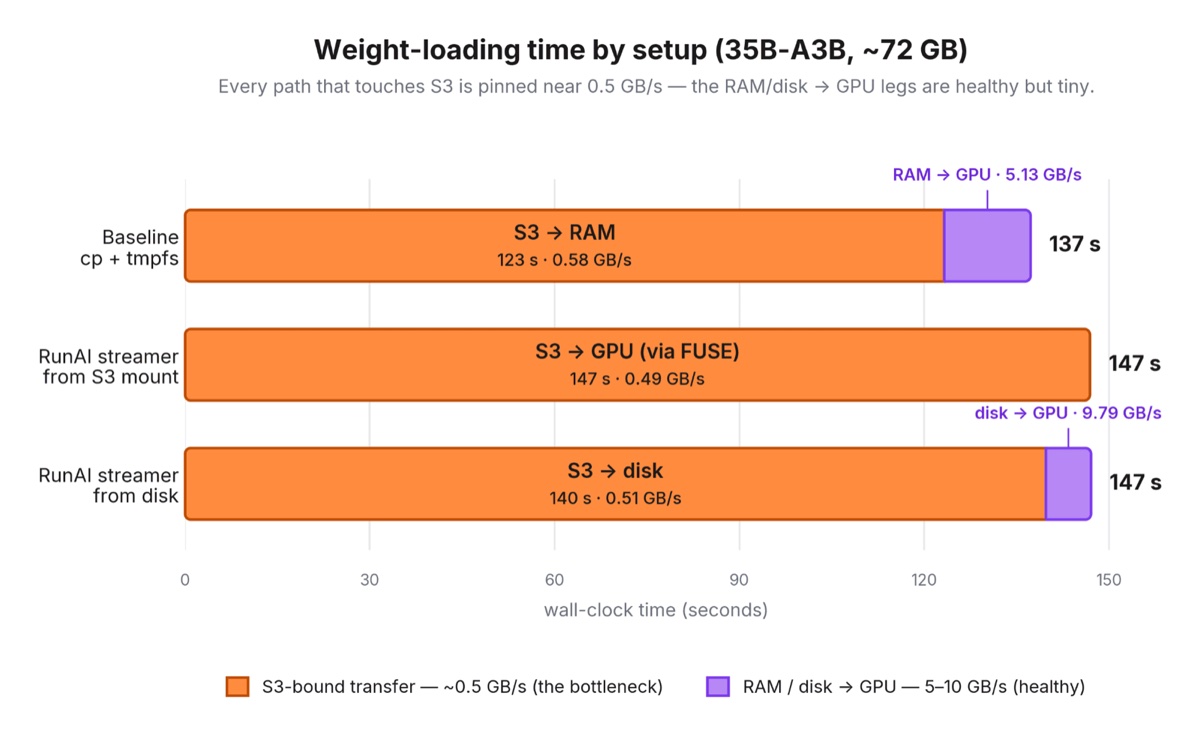
We benchmarked three configurations to isolate the bottleneck: our standard cp baseline, the ModelExpress loader streaming directly from the S3 FUSE mount, and the same streamer reading from local RAM after a pre-stage step.
 (opens full size in a new tab)
Weight-loading time by setup for the 35B-A3B model.
The data points to a clear structural limit:
- Local transfers perform well: RAM-to-GPU and disk-to-GPU copies move data quickly, hovering between 5 GB/s and 10 GB/s.
- The S3 boundary is a hard bottleneck: Every code path that pulls directly from S3 stalls out near 0.5 GB/s.
- Client logic does not solve network caps: This 25x performance gap remains completely unchanged whether we use single-threaded
cpcommands or parallel, multi-threaded streamers.
Experiment 2: Optimizing S3 mount configuration
When we investigated the low S3 throughput, we found that our mount-s3 processes were running with stock default settings. The container logs revealed that the system failed to detect our specific instance capabilities, causing it to drop to a 10 Gbps baseline network cap.
WARN mountpoint_s3::cli: failed to detect network throughput. Using 10 gbps as throughput.
Use --maximum-throughput-gbps CLI flag to configure a target throughput appropriate for
the instance. Detection failed due to: failed to get instance type: IMDS query failed:
Unknown CRT error
Mountpoint-S3 determines its client settings by hitting the EC2 Instance Metadata Service (IMDS) for the specific instance type. Inside our pods, this IMDS query timed out. The failure forced a 10 Gbps throughput cap and standard 8 MB read parts onto every weight loading path in the cluster. We fixed this by hardcoding two mount options into our CDK Persistent Volume (PV) configuration:
const pv = cluster.addManifest(options.cfnPvId, {
  // ... metadata and spec ...
  mountOptions: [
    `region ${options.region}`,
    // Explicit throughput target, bypasses the IMDS auto-detect that
    // fails fleet-wide and falls back to a generic 10 Gbps.
    'maximum-throughput-gbps 100',
    // 32 MB parts vs the 8 MB default, cuts S3 request count 4x and
    // amortizes per-request overhead (crucial for many-small-shard fp8 models).
    'read-part-size 33554432',
  ],
  // ... CSI driver config ...
});
After updating the configuration, we ran the benchmarks again. While cp showed a tiny bump from 0.58 to 0.67 GB/s, the RunAI streamer nearly doubled its speed, climbing from 0.49 to 0.94 GB/s. This was progress, but we were still an order of magnitude away from our 12.5 GB/s target.
The low cp improvement shows a clear network ceiling. Because cp is single threaded, it relies on a single TCP flow. AWS enforces a hard cap of 5 Gbps (0.625 GB/s) on single-flow traffic, no matter the instance type. Reaching 0.67 GB/s means we hit the physical limit for a single-threaded copy on AWS. We could not get any faster without adding parallelism.
Experiment 3: Escaping the FUSE bottleneck
Even with parallel threads, the RunAI streamer maxes out at 0.94 GB/s. This limit comes from the FUSE architecture, which forces every byte through multiple user-kernel space transitions:
- VFS execution: Application threads trigger parallel reads through the kernel Virtual File System (VFS).
- Driver transition: The kernel forwards these requests to the FUSE driver.
- Context switch: The system runs a context switch to pass data to the Mountpoint daemon in userspace.
- Memory copying: Mountpoint runs S3 HTTP requests and copies the data back across the user-kernel boundary.
Processing 72 GB through this pipeline maxes out the FUSE daemon's CPU cores long before it can fill the network pipe. Because FUSE exposes the bucket as a POSIX filesystem, it also blocks the streamer's native parallel S3 client from running correctly.
Establishing a Baseline Performance Ceiling
To isolate FUSE overhead from raw S3 performance, we bypassed the mount completely and downloaded the 14 shards straight to /dev/shm via the AWS CLI:
| Tool / Configuration | Avg Throughput | Peak (sar, eth0) |
|---|---|---|
aws s3 cp, default (10 conc / 8 MB parts) | 0.36 GB/s | ~0.40 GB/s |
aws s3 cp, tuned (64 conc / 64 MB parts) | 0.41 GB/s | ~0.46 GB/s |
aws s3 cp, CRT client, 100 Gbps target | 3.75 GB/s | ~6.0 GB/s |
| 14 parallel single-shard CRT processes | 2.22 GB/s | ~4.6 GB/s |
The benchmarks show the standard Python based CLI hits a CPU ceiling at 0.4 GB/s. Moving to the CRT optimized C client gives a 10x performance boost, peaking near 6 GB/s. That gets us to 50% of the theoretical NIC limit and establishes our target download speed at 3.75 GB/s.
Bypassing FUSE for Direct S3 Access
We verified the FUSE bottleneck by pointing the RunAI streamer directly at the bucket (s3://) and scaling read concurrency:
| Streamer Configuration | Throughput | vs. PVC Baseline |
|---|---|---|
| Via mount-s3 PVC | 0.94 GB/s | N/A |
| Direct bucket (conc. 1) to RAM | 0.82 GB/s | ~1x |
| Direct bucket (conc. 2) to RAM | 1.49 GB/s | ~1.8x |
| Direct bucket (default) to GPU | 1.78 GB/s | ~2.2x |
While direct access at concurrency 1 matches FUSE performance, only the direct path scales up as concurrency increases. Bypassing the FUSE layer completely lets the streamer communicate directly with S3 without blocking user-kernel transitions.
Experiment 4: Distributing the download across the node's GPUs
The optimizations up to this point handled a single download stream. However, our large models run with tensor parallelism (TP) across all 8 GPUs of a node, highlighting a different bottleneck.
Under standard TP, each GPU only keeps a 1/N slice of the weights (about 50 GB for the 397B model). The problem is how the default loader handles the transfer:
- The redundant download problem: Every GPU worker streams the full model bytes from S3, reading entire tensors just to slice out its specific share and throwing away the rest. This pulls 3.2 TB over the network for a 400 GB model, forcing 8 workers to fight for the same NICs and CPU cores.
- The distributed streaming solution: Each of the 8 GPUs downloads a unique 1/8th chunk of the shards from S3 in parallel. The workers then route those pieces across the 900 GB/s intra-node NVLink and NVSwitch fabric using an NCCL all-gather, reading the model from S3 exactly once and cutting the per-GPU network demand by 8x.
This distributed setup runs natively in the RunAI model streamer via its is_distributed mode. Inside ModelExpress, we toggle this on using enable_distributed_streaming (setting MX_MS_DISTRIBUTED=1).
We tested this on our largest configuration: the Qwen3.5-VL-397B-A17B FP8 model (~409 GB) on a full 8-GPU TP8 node. This cluster was the worst casualty of the redundant download loop that caused our original 11 minute delay.
We measured the following results:
| Configuration (397B FP8, TP8) | Weight loading time | Throughput |
|---|---|---|
| S3 FUSE mount | 9.9 min (593 s) | ~0.69 GB/s* |
| Direct bucket, concurrency 16 | 14.9 min (892 s) | ~0.46 GB/s* |
| Direct bucket, distributed | 3.4 min (204 s) | ~2.0 GB/s* |
* Note: Further tuning of the model streamer configuration should fully saturate the potential S3 bandwidth and could improve performance even further.
The naive direct bucket path turned out to be the slowest configuration. At TP8, the 8 redundant downloads caused so much network and hardware contention that performance dropped below the baseline FUSE mount. Meanwhile, distributed streaming reads the model once and redistributes it via NVLink, running 3x faster than the mount and 4x faster than naive concurrency.
Wrap-up
Distributed streaming cuts the 397B FP8 weight pull from around 11 minutes down to 3.4 minutes. This 3x speedup means weight staging is no longer the main bottleneck holding up a cold start.
By pairing direct bucket access and mount tuning with distributed streaming, weight loading is now limited only by how fast the node's network cards can pull a single copy of the model. We completely wiped out the overhead from the FUSE layer and duplicate per-GPU downloads.
Layer 3: Leveraging Peer-to-Peer Weight Distribution
Once the first model replica is active, pulling the same weights from S3 for subsequent instances is a waste of bandwidth. Those weights are already inside the cluster, sitting in a neighbor's GPU memory and connected by high-speed hardware.
To use this, we set up the RDMA loading strategy from ModelExpress as a hot path for vLLM scale-out operations:
- Peer discovery: The engine queries the ModelExpress gRPC server to identify host GPUs that already hold the target model.
- Peer-to-peer transfer: If a peer matches, weights migrate GPU to GPU over RDMA using NIXL, libfabric, and AWS EFA, completely skipping host RAM and S3.
- Optimized fallback: Only the initial replica goes through an S3 cold start. Every replica after that fetches weights from peers at maximum fabric line speed.
 (opens full size in a new tab)
ModelExpress transfers 62 GB between GPU replicas in 1.4 seconds at 341 Gbps.
The "RDMA" Illusion
Our initial tests on a 4B model were surprisingly slow. The RDMA path clocked in at 1.8 Gbps, moving 9.21 GB in 39 seconds, which was actually slower than our optimized S3 streaming. On a P5 instance equipped with EFA, it was clear we weren't hitting the hardware fabric.
The problem was inside the userspace transport stack. AWS provides two paths to EFA hardware:
- Libfabric: the AWS optimized path used by NCCL.
- Libibverbs: the standard Linux RDMA API.
Our loader relied on NIXL with a UCX backend via libibverbs. While the nixl-cu12 wheel bundles libibverbs v48, our nodes use AWS EFA providers built for v55+. This ABI mismatch prevented the bundled library from binding to the EFA device, causing a silent fallback to standard TCP over Ethernet.
Aligning with the NCCL Path
To bypass libibverbs versioning issues, we transitioned NIXL to its LIBFABRIC backend. This allows it to ignore the bundled library and interface directly with the system path at /opt/amazon/efa/lib/libfabric.so.1. We have since upstreamed this option to ModelExpress.
The performance gains were immediate:
| Metric | UCX to TCP | Libfabric to EFA | Speedup |
|---|---|---|---|
| Wire transfer | 41.40 s | 0.22 s | 188x |
| Throughput | 1.8 Gbps | 341 Gbps | 189x |
| Total model load | 41.05 s | 3.85 s | 10.6x |
The performance scaling holds up at baseline. In a test using our 122B-A10B MoE model with TP=4, each worker pulled its 62 GB shard from a peer in roughly 1.4 seconds, averaging a throughput of 340 Gbps per worker:
[Worker 3] RDMA transfer complete: 1118 tensors, 62.17 GB, 1.424s, 349.3 Gbps
[Worker 2] RDMA transfer complete: 1118 tensors, 62.17 GB, 1.422s, 349.8 Gbps
[Worker 0] RDMA transfer complete: 1118 tensors, 62.17 GB, 1.473s, 337.6 Gbps
[Worker 1] RDMA transfer complete: 1118 tensors, 62.17 GB, 1.471s, 338.0 Gbps
Layer 4: Warmup, compile once, reuse everywhere
Even with images cached and weights moving at fabric speeds, warmup is still a massive bottleneck. This is worst on FP8 models, where JIT compilation for DeepGEMM kernels can keep a server from handling traffic for up to 10 minutes.
vLLM does save compilation data, including Inductor artifacts, compiled Triton kernels, the torch.compile graph, and DeepGEMM JIT kernels. The problem is that these caches are purely local. Every replica landing on a new node has to recompile the exact same kernels for the identical hardware and model setup.
We fixed this by turning these local files into a shared artifact using three design rules:
- Deterministic cache identity: We use a hash of all compilation-affecting variables, such as GPU type, model path, quantization, and TP/PP sizes, to generate a cache ID. This makes sure deployments pull the correct cache and prevents corruption if the config changes.
- Leader election: To stop multiple nodes from writing at the same time, an init container uses a Kubernetes Lease or a shared storage lock to choose a leader. The leader builds the cache while the other replicas wait, using a heartbeat system so a follower can take over if the leader fails.
- Persistence: Once vLLM passes its health checks, a sidecar saves the cache to a shared file system. Future deployments grab this cache before the engine even initializes.
The startup numbers show a clear speedup, especially since the cache files are a fraction of the size of the actual weights.
| Model (fp8) | Cold boot | Warm boot (vLLM cache available) | Cache size |
|---|---|---|---|
| 8B | 6:45 | 1:37 | 236 MB |
| 32B | 8:42 | 2:26 | 822 MB |
| 30B-A3B | 12:54 | 2:35 | 1.0 GB |
| 235B-A22B | 14:56 | 4:53 | 8.5 GB |
Putting it all together
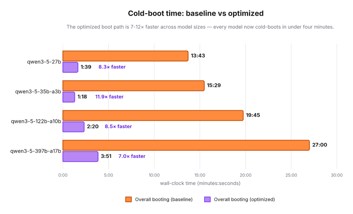
By combining all four optimization layers (the image cache, accelerated S3 staging, P2P weight distribution, and distributed compilation caches) we achieve the following end-to-end boot times in the warm start setup.
 (opens full size in a new tab)
Cold-boot time: baseline versus optimized.
While larger models still take a bit longer to boot than smaller ones, we are making massive strides. By optimizing our data handling across the board, we have effectively removed the data-transfer bottleneck. The startup time is now primarily determined by the fixed overhead of initializing the engine and preparing the GPU, rather than the size of the model itself.
Wrap up & next steps
We fixed our inference fleet boot times by treating cluster startup as an ordinary optimization problem instead of a fixed tax. By swapping out default, choked network paths for DaemonSet caching, direct S3 streaming, RDMA peer transfers, and shared JIT compilation caches, we stopped model size from dictating our boot latency. The system now delivers predictable, fast starts so our agents can scale out without the massive delay.
We want to thank the ModelExpress maintainers for their responsiveness, and the vLLM community for integrating our startup-tracing improvements.
Next steps
While this post focused on the boot path, these optimizations are already fueling our next phase of work:
- Reactive autoscaling: now that node startup is fast, we updated our cluster policies to cut down on idle over-allocation. We can now spin up capacity on the fly to handle sudden spikes in agent traffic without wasting GPU time.
- Process Snapshotting: to bypass the remaining software initialization delays like Python imports and internal vLLM configuration, we are testing memory snapshotting. We want to restore pre-initialized processes from memory to hit an instant warm boot.
If chasing hardware-limit performance across the inference stack sounds like fun, we're hiring.